Angelique's GIS Portfolio

In this week's lab, I classified satellite imagery using unsupervised and supervised classification methods in ERDAS Imagine. For the supervised classification, I created spectral signatures for 8 classes in Germantown, Maryland using the Region Growing Properties tool, Polygon tool, and the Signature Editor tool. After creating several Areas of Interests (AOIs) for each class, I examined the histograms and mean plots of all the signatures for spectral confusion. Based on the histograms and plots, I concluded that bands 4, 5, and 6 were the most separate and least confused of all the signatures. I used these bands for the supervised classification using Maximum Likelihood. I recoded the supervised image to merge the AOIs into 8 classes and calculated the area in acres for each of the classes. Below is the final result of supervised classification.  Fig 1. Land use map from supervised classification of Germantown, Maryland.

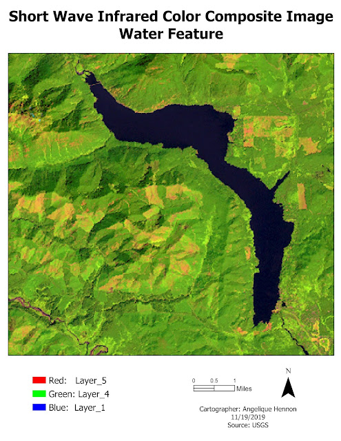
The deliverables for this lab included identifying three features from pixel descriptions on an image in ERDAS Imagine. Grayscale and Multispectral versions of the image were examined using layer histograms and the Inquire Cursor. Once the feature was identified, the Create Subset tool was used to create an image of the area to import into ArcGIS Pro to create the maps. A different multispectral band combination was used for each feature mapped to make that feature stand out. The maps below show each of the features identified in the lab. The water features in the image produced a spike between pixel values of 12 to 18 in Layer_4. To make the feature stand out and identifiable as blue water, Short Wave Infrared Color Composite band combination was selected where dark blue is water, green is vegetation and pink is bare soil. The snow in the image produced both a small spike around pixel value 200 in Layers 1-4 and a large spike between pixel values 9 and 11 in Layers 5-6. To m...

In this week's lab, I learned basic tools and functions for exploring imagery in ERDAS Imagine. ERDAS Imagine is pretty similar to ArcGIS Pro in terms of the way the system is setup for navigating and exploring layers, so learning to use the new software was fairly easy. I used ERDAS Imagine to select an area from a classified image of some forested lands in Washington State. Before saving the file, I added a new column with the area in hectares of each cover type in the image. Adding the area column was easier and took fewer steps in ERDAS Imagine than it would have in ArcGIS Pro. I saved the selected area as an .img file and then opened it in ArcGIS Pro to create a map with a legend, including the area of each cover type calculated in ERDAS Imagine. Fig 1. Map of forested land cover types in Washington State derived from a classified image in ERDAS Imagine. 

In this week's lab, I practiced feature recognition skills using natural color aerial photography by digitizing an area of Pascagoula, MS to create a land use/land cover map in ArcGIS Pro. To do this, I used a USGS Standard Land Use / Land Cover Classification Scheme and digitized polygons to Level II based on features in the landscape. For each of the classification codes, I developed a guide with recognition elements to aid in the LULC classification. Once the classification was complete, I used the Create Random Sample tool in ArcGIS Pro to create 30 ransom points within the area. I then used Google maps street view to "ground truth" these locations to check the accuracy of my LULC classifications. Fig 1. LULC map of an area of Pascagoula, MS digitized to Level II of the USGS Standard LULC Classification Scheme showing the accuracy of 30 randomly generated ground truthing locations.